December | 2017 | Topics in Probability

A great number of problems involving Markov chains can be evaluated by a technique called first step analysis. The general idea of the method is to break down the possibilities resulting from the first step (first transition) in the Markov chain. Then use the law of total probability and Markov property to derive a set of relationship among the unknown variables. This technique is demonstrated in this previous post in several examples. In this post, the technique is further discussed. An alternative approach based on the fundamental matrix is also emphasized.

This previous post shows how to use first step analysis to solve two problems: to determine the probability of absorption from transient states and to determine the expected time spent in transient states. This post shows that first step analysis leads to an effective approach of using fundamental matrix for solving the same two problems. We illustrate using an example.

Illustrative Example

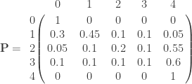
We start with Example 3 discussed in the previous post. It involves the following transition probability matrix.

$\mathbf{P} = \bordermatrix{ & 0 & 1 & 2 & 3 & 4 \cr 0 & 1 & 0 & 0 & 0 & 0 \cr 1 & 0.4 & 0.3 & 0.1 & 0.1 & 0.1 \cr 2 & 0.1 & 0.1 & 0.5 & 0.2 & 0.1 \cr 3 & 0.1 & 0.2 & 0.1 & 0.5 & 0.1 \cr 4 & 0 & 0 & 0 & 0 & 1 \cr } \qquad$

The Markov chain represented by $\mathbf{P}$ cycles through 5 states. Whenever the process reaches state 0 or state 4, it stays there and not move. These two states are called absorbing states. The other states (1, 2 and 3) are called transient states because the process stays in each of these states a finite amount of time. When the process starts at one of these states, it will eventually transition (be absorbed) into one of the absorbing states (0 or 4). Thus the matrix $\mathbf{P}$ is called an absorbing Markov chain.

A natural question: how likely that the process is absorbed into state 0 versus state 4? Of course the answer to this question depends on the starting state.

Another question: if starting at state 1, 2 or 3, how many steps on average it will take for the process to be absorbed? In other words, what is the mean time to absorption? Of course, the answer will depend on the starting state.

Let $T$ the time it takes the process to be absorbed into 0 or 4. More specifically let $T$ be defined by $T=\{ n \ge 0: X_n=0 \text{ or } X_n=4 \}$ . If the starting state is $i$ , let $U_i$ be the probability of the process being absorbed into state 0 and let $V_i$ be the expected time to absorption (into state 0 or state 4). The quantities $U_i$ and $V_i$ can also be defined as follows:

$U_i=P[X_T=0 \lvert X_0=i] \ \ \ \ i=1,2,3$

$V_i=E[T \lvert X_0=i] \ \ \ \ \ \ \ \ \ \ i=1,2,3$

The quantities $U_i$ are the probabilities of absorption into state 0 and the quantities $V_i$ are the expected times to absorption (from each transient state). Applying the first step analysis produces the following two sets of equations.

$\displaystyle \begin{aligned}&U_1=0.4+0.3 \times U_1+0.1 \times U_2+0.1 \times U_3 \\&U_2=0.1+0.1 \times U_1+0.5 \times U_2+0.2 \times U_3 \\&U_3=0.1+0.2 \times U_1+0.1 \times U_2+0.5 \times U_3 \end{aligned}$

$\displaystyle \begin{aligned}&V_1=1+0.3 \times V_1+0.1 \times V_2+0.1 \times V_3 \\&V_2=1+0.1 \times V_1+0.5 \times V_2+0.2 \times V_3 \\&V_3=1+0.2 \times V_1+0.1 \times V_2+0.5 \times V_3 \end{aligned}$

We rearrange the equations by putting the variables $U_i$ or $V_i$ on one side and the constant terms on the other side.

$\displaystyle \begin{array}{rcr} \displaystyle 0.7 \times U_1-0.1 \times U_2-0.1 \times U_3 & = & 0.4 \\ \displaystyle -0.1 \times U_1+0.5 \times U_2-0.2 \times U_3 & = & 0.1 \\ \displaystyle -0.2 \times U_1-0.1 \times U_2+0.5 \times U_3 & = & 0.1 \end{array} \ \ \ \ \ \ \ \ \ \ \ \ \ \ \ \ \ \ (1a)$

$\displaystyle \begin{array}{rcr} \displaystyle 0.7 \times V_1-0.1 \times V_2-0.1 \times V_3 & = & 1 \\ \displaystyle -0.1 \times V_1+0.5 \times V_2-0.2 \times V_3 & = & 1 \\ \displaystyle -0.2 \times V_1-0.1 \times V_2+0.5 \times V_3 & = & 1 \end{array} \ \ \ \ \ \ \ \ \ \ \ \ \ \ \ \ \ \ \ \ \ (2a)$

The probabilities of absorption into state 0 are found by solving the system of equations (1a). The mean times to absorption are found by solving the system of equations (2a). It will be informative to write (1) and (2) in matrix notations.

$\left[\begin{array}{rrr} 0.7 & -0.1 & -0.1 \\ -0.1 & 0.5 & -0.2 \\ -0.2 & -0.1 & 0.5 \end{array}\right] \left[\begin{array}{c} U_1 \\ U_2 \\ U_3 \end{array}\right] = \left[\begin{array}{c} 0.4 \\ 0.1 \\ 0.1 \end{array}\right] \ \ \ \ \ \ \ \ \ \ \ \ \ \ \ \ \ \ (1b)$

$\left[\begin{array}{rrr} 0.7 & -0.1 & -0.1 \\ -0.1 & 0.5 & -0.2 \\ -0.2 & -0.1 & 0.5 \end{array}\right] \left[\begin{array}{c} V_1 \\ V_2 \\ V_3 \end{array}\right] = \left[\begin{array}{c} 1 \\ 1 \\ 1 \end{array}\right] \ \ \ \ \ \ \ \ \ \ \ \ \ \ \ \ \ \ \ \ (2b)$

Note that the same matrix appears on the left side of both (1b) and (2b). The quantities $U_i$ and $V_i$ can be found by multiplying both sides by the following inverse matrix.

$\left[\begin{array}{rrr} 0.7 & -0.1 & -0.1 \\ -0.1 & 0.5 & -0.2 \\ -0.2 & -0.1 & 0.5 \end{array}\right]^{-1}=\left[\begin{array}{rrr} 230/141 & 60/141 & 70/141 \\ 90/141 & 330/141 & 150/141 \\ 110/141 & 90/141 & 340/141 \end{array}\right]$

Multiplying (1b) and (2b) by the inverse matrix produces the following.

$\left[\begin{array}{c} U_1 \\ U_2 \\ U_3 \end{array}\right] = \left[\begin{array}{rrr} 230/141 & 60/141 & 70/141 \\ 90/141 & 330/141 & 150/141 \\ 110/141 & 90/141 & 340/141 \end{array}\right] \times \left[\begin{array}{c} 0.4 \\ 0.1 \\ 0.1 \end{array}\right] =\left[\begin{array}{c} 35/47 \\ 28/47 \\ 29/47 \end{array}\right]=\left[\begin{array}{c} 0.745 \\ 0.596 \\ 0.617 \end{array}\right] \ \ \ \ \ \ \ \ \ \ \ \ \ \ \ \ (1c)$

$\left[\begin{array}{c} V_1 \\ V_2 \\ V_3 \end{array}\right] = \left[\begin{array}{rrr} 230/141 & 60/141 & 70/141 \\ 90/141 & 330/141 & 150/141 \\ 110/141 & 90/141 & 340/141 \end{array}\right] \times \left[\begin{array}{c} 1 \\ 1 \\ 1 \end{array}\right] =\left[\begin{array}{c} 360/141 \\ 570/141 \\ 540/141 \end{array}\right]=\left[\begin{array}{c} 2.55 \\ 4.04 \\ 3.83 \end{array}\right] \ \ \ \ \ \ \ \ \ \ \ \ \ \ \ \ \ (2c)$

The systems of equations (1a) and (2a) can certainly be solved by using other methods (e.g. Gaussian elimination). The inverse matrix approach is clean and can be implemented using software. More importantly, using the inverse matrix leads to a general description of the algorithm based on fundamental matrix.

How is the matrix in (1b) and (2b) obtained? Recall that the equations in (1a) and (2a) are obtained by rearranging the equations from the first step analysis. The first step analysis is of course based on the original transition probability matrix $\mathbf{P}$ . The matrix in question is obtained from the transition probability matrix $\mathbf{P}$ . The next two sections show how.

More about the Example

Before stating the algorithm, we continue to use the above example as illustration. The following is a rewrite of the transition probability matrix $\mathbf{P}$ . Note that the transient states are grouped together.

$\mathbf{P} = \bordermatrix{ & 1 & 2 & 3 & \text{ } & 0 & 4\cr 1 & 0.3 & 0.1 & 0.1 & \text{ } & 0.4 & 0.1 \cr 2 & 0.1 & 0.5 & 0.2 & \text{ } & 0.1 & 0.1 \cr 3 & 0.2 & 0.1 & 0.5 & \text{ } & 0.1 & 0.1 \cr \text{ } & \text{ } & \text{ } & \text{ } & \text{ } & \text{ } & \text{ } \cr 0 & 0 & 0 & 0 & \text{ } & 1 & 0 \cr 4 & 0 & 0 & 0 & \text{ } & 0 & 1 \cr } \qquad=\left[\begin{array}{rr} Q & R \\ \mathbf{0} & I \\ \end{array}\right]$

The matrix $Q$ is the 3 x 3 matrix of transition probabilities for the 3 transient states 1, 2 and 3. The matrix $Q$ describes the transition probabilities between transient states. The matrix $R$ is a 3 x 2 matrix that shows the transition probabilities from transient to absorbing states. The matrix $\mathbf{0}$ is a 2 x 3 matrix consisting of 0’s. The matrix $I$ is an identity matrix describing the absorbing states (in this case 2 x 2).

The key matrix is the matrix $I-Q$ where $I$ is a 3 x 3 identity matrix.

$I-Q=\left[\begin{array}{rrr} 1 & 0 & 0 \\ 0 & 1 & 0 \\ 0 & 0 & 1 \end{array}\right]-\left[\begin{array}{rrr} 0.3 & 0.1 & 0.1 \\ 0.1 & 0.5 & 0.2 \\ 0.2 & 0.1 & 0.5 \end{array}\right]=\left[\begin{array}{rrr} 0.7 & -0.1 & -0.1 \\ -0.1 & 0.5 & -0.2 \\ -0.2 & -0.1 & 0.5 \end{array}\right]$

The matrix $W=(I-Q)^{-1}$ , the inverse of $I-Q$ , is called the fundamental matrix for the absorbing chain in question. As shown above, the fundamental matrix is used in finding the probabilities of absorption and the mean times to absorption.

The Algorithm

Recall that an absorbing Markov chain has at least one absorbing state such that every non-absorbing state will eventually transition into an absorbing state (i.e. will eventually be absorbed). The non-absorbing states in such a chain are called transient states.

Consider an absorbing Markov chain with transition probability matrix $\mathbf{P}$ . Suppose that the chain has $N+1$ states with transient states $0,1,2,\cdots,y-1$ and absorbing states $y,y+1,\cdots,N$ . Such labeling is for convenience. As the above example shows, the rearranging of the states is not necessary as long as one can keep the transient states apart from the absorbing states.

Write the matrix $\mathbf{P}$ in the following form

$\mathbf{P}=\left[\begin{array}{rr} Q & R \\ \mathbf{0} & I \\ \end{array}\right]$

where $Q$ consists of $P_{ij}$ where $0 \le i,j \le y-1$ and $R$ consists of $P_{ij}$ where $0 \le i \le y-1$ and $y \le j \le N$ . In other words, the matrix $Q$ contains the one-step transition probabilities between transient states and $R$ contains the one-step transition probabilities from transient states into absorbing states. The matrix $\mathbf{0}$ is a $(N+1-y) \times y$ matrix consisting of 0’s. The matrix $I$ is an $(N+1-y) \times (N+1-y)$ identity matrix describing the absorbing states.

Consider the matrix $I-Q$ where $I$ is the $y \times y$ identity matrix. Then $W=(I-Q)^{-1}$ , the inverse of $I-Q$ , is the fundamental matrix for the absorbing Markov chain.

Here is one important property of the matrix $W=[ W_{ij} ]$ .

An element $W_{ij}$ of $W$ represents the total time the chain spends in the transient state $j$ if the starting state is the transient state $i$ .

This leads to the following observation.

The sum of all entries in a row of $W$ is the total time the chain is expected to spend in all the transient states if the starting state is the transient state corresponding to that row.

Here’s the property concerning probability of absorption.

The matrix $U=W \times R$ , the product of the matrix $W$ and the matrix $R$ , gives the probabilities of absorption. For example, the element $U_{ij}$ of $U$ is the probability of being absorbed into the state $j$ if the starting state is $i$ .

To make the mathematical properties even more precise, consider $T=\{ n \ge 0: y \le X_n \le N \}$ . The variable $T$ is the random number of steps the process takes to reach an absorbing state. Define the following quantities.

$U_{ij}=P[T=j \lvert X_0=i]$

$V_{i}=E[T \lvert X_0=i]$

where $i$ is any transient state ( $0 \le i \le y$ ) and $j$ is any absorbing state ( $y \le j \le N$ ). Here’s how to tie $U_{ij}$ and $V_i$ to the above stated facts.

The quantity $V_i$ is simply the sum of all entries of the row corresponding to the transient state $i$ in the matrix $W$ . Equivalently let $\mathbf{V}$ be the column vector with entries $V_i$ . Then $\mathbf{V}=W \times \mathbf{1}$ where $\mathbf{1}$ is the column vector consisting of all 1’s.

The quantities $U_{ij}$ are simply the entries in the matrix $U=W \times R$ .

To further illustrate the technique, the next section has examples. It is critical that calculator or software be available for computing inverse matrix. Here is a useful online matrix calculator.

Examples

Example 1
This is another calculation example to illustrate the technique. Use the following transition probability matrix to compute the quantities $U_{ij}=P[T=j \lvert X_0=i]$ (the probabilities of being absorbed into states 0 and 4) and $V_{i}=E[T \lvert X_0=i]$ (the expected time spent in transient states 1,2 and 3 given the starting state is $i$ ). Of course $T$ is the random time to absorption defined by $T=\{ n \ge 0: X_n=0 \text{ or } X_n=4 \}$ .

$\mathbf{P} = \bordermatrix{ & 0 & 1 & 2 & 3 & 4 \cr 0 & 1 & 0 & 0 & 0 & 0 \cr 1 & 0.3 & 0.45 & 0.1 & 0.1 & 0.05 \cr 2 & 0.05 & 0.1 & 0.2 & 0.1 & 0.55 \cr 3 & 0.1 & 0.1 & 0.1 & 0.1 & 0.6 \cr 4 & 0 & 0 & 0 & 0 & 1 \cr } \qquad$

The following shows the matrices that are used in calculation.

$Q = \bordermatrix{ & 1 & 2 & 3 \cr 1 & 0.45 & 0.1 & 0.1 \cr 2 & 0.1 & 0.2 & 0.1 \cr 3 & 0.1 & 0.1 & 0.1 \cr } \qquad \ \ \ \ R = \bordermatrix{ & 0 & 4 \cr 1 & 0.3 & 0.05 \cr 2 & 0.05 & 0.55 \cr 3 & 0.1 & 0.6 \cr } \qquad$

$I-Q=\left[\begin{array}{rrr} 0.55 & -0.1 & -0.1 \\ -0.1 & 0.8 & -0.1 \\ -0.1 & -0.1 & 0.9 \end{array}\right]$

$W=(I-Q)^{-1}=\left[\begin{array}{rrr} 1420/743 & 200/743 & 180/743 \\ 200/743 & 970/743 & 130/743 \\ 180/743 & 130/743 & 860/743 \end{array}\right]$

Here’s the matrix calculation to obtain the desired quantities.

$\left[\begin{array}{r} V_1 \\ V_2 \\ V_3 \end{array}\right]=\left[\begin{array}{rrr} 1420/743 & 200/743 & 180/743 \\ 200/743 & 970/743 & 130/743 \\ 180/743 & 130/743 & 860/743 \end{array}\right] \times \left[\begin{array}{r} 1 \\ 1 \\ 1 \end{array}\right]=\left[\begin{array}{r} 2.4226 \\ 1.7497 \\ 1.5747 \end{array}\right]$

$U=W \times R=\left[\begin{array}{rr} 908/1486 & 578/1486 \\ 243/1486 & 1243/1486 \\ 293/1486 & 1193/1486 \end{array}\right]=\left[\begin{array}{rr} 0.6110 & 0.3890 \\ 0.1635 & 0.8365 \\ 0.1972 & 0.8028 \end{array}\right]=\left[\begin{array}{rr} U_{1,0} & U_{1,4} \\ U_{2,0} & U_{2,4} \\ U_{2,0} & U_{3,4} \end{array}\right]$

Example 2
A fair coin is tossed repeatedly until the appearance of 4 consecutive heads. Determine the mean number of tosses required.

Consider the 5-state Markov chain with states 0, H, HH, HHH and HHHH. The state 0 means that the last toss is not a head. These 5 states are labeled 0, 1, 2, 3, 4 and 5, respectively.

$\mathbf{P} = \bordermatrix{ & 0 & \text{1=H} & \text{2=HH} & \text{3=HHH} & \text{4=HHHH} \cr 0 & 0.5 & 0.5 & 0 & 0 & 0 \cr 1 & 0.5 & 0 & 0.5 & 0 & 0 \cr 2 & 0.5 & 0 & 0 & 0.5 & 0 \cr 3 & 0.5 & 0 & 0 & 0 & 0.5 \cr 4 & 0 & 0 & 0 & 0 & 1 \cr } \qquad$

Note that when a toss results in a tail, the process bounces back to the state 0. Otherwise, it advances to the next state (e.g. HH to HHH). The transient states are 0, 1, 2 and 3. State 4 is the absorbing state. The natural question is: on average how many tosses does it take to reach state 4 (to get 4 consecutive heads)? It is informative to obtain the matrix $I-Q$ and to find its inverse.

$I-Q=\left[\begin{array}{rrrr} 1 & 0 & 0 & 0 \\ 0 & 1 & 0 & 0 \\ 0 & 0 & 1 & 0 \\ 0 & 0 & 0 & 1 \end{array}\right]-\left[\begin{array}{rrrr} 0.5 & 0.5 & 0 & 0 \\ 0.5 & 0 & 0.5 & 0 \\ 0.5 & 0 & 0 & 0.5 \\ 0.5 & 0 & 0 & 0 \end{array}\right]=\left[\begin{array}{rrrr} 0.5 & -0.5 & 0 & 0 \\ -0.5 & 1 & -0.5 & 0 \\ -0.5 & 0 & 1 & -0.5 \\ -0.5 & 0 & 0 & 1 \end{array}\right]$

$(I-Q)^{-1} = \bordermatrix{ & 0 & \text{1=H} & \text{2=HH} & \text{3=HHH} \cr 0 & 16 & 8 & 4 & 2 \cr 1 & 14 & 8 & 4 & 2 \cr 2 & 12 & 6 & 4 & 2 \cr 3 & 8 & 4 & 2 & 2 \cr } \qquad$

The sum of the first row of $(I-Q)^{-1}$ is 30. It takes on average 30 tosses to get 4 consecutive heads if starting from scratch. After getting the first head, the process spends on average 28 tosses (the sum of the second row) before getting 4 consecutive heads. Even with three consecutive heads obtained, the chain still spends on average 16 tosses before reaching the state HHHH! On the surface, this may seem unbelievable. Remember that whenever a toss results in a tail, the process reverts back to 0 and the process essentially starts over again.

Example 3 (Occupancy Problem)
This example revisits the occupancy problem, which is discussed here. The occupancy problem is a classic problem in probability. The setting of the problem is that $k$ balls are randomly distributed into $N$ cells (or boxes or other containers) one at a time. After all the $k$ balls are distributed into the cells, we examine how many of the cells are occupied with balls. In this particular example, the number of balls is not fixed. Instead, balls are thrown into the cells one at a time until all cells are occupied. On average how many balls have to be thrown to achieve this?

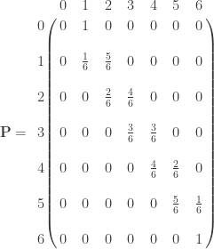
More specifically, let $n=6$ (cells). On average, how many balls have to be thrown until all 6 cells are occupied? Let $X_n$ be the number of occupied cells after $n$ balls are thrown. The following is the transition probability matrix describing this Markov chain.

$\displaystyle \mathbf{P} = \bordermatrix{ & 0 & 1 & 2 & 3 & 4 & 5 & 6 \cr 0 & 0 & 1 & 0 & 0 & 0 & 0 & 0 \cr \text{ } & \text{ } & \text{ } & \text{ } & \text{ } & \text{ } & \text{ } & \text{ } \cr 1 & 0 & \frac{1}{6} & \frac{5}{6} & 0 & 0 & 0 & 0 \cr \text{ } & \text{ } & \text{ } & \text{ } & \text{ } & \text{ } & \text{ } & \text{ } \cr 2 & 0 & 0 & \frac{2}{6} & \frac{4}{6} & 0 & 0 & 0 \cr \text{ } & \text{ } & \text{ } & \text{ } & \text{ } & \text{ } & \text{ } & \text{ } \cr 3 & 0 & 0 & 0 & \frac{3}{6} & \frac{3}{6} & 0 & 0 \cr \text{ } & \text{ } & \text{ } & \text{ } & \text{ } & \text{ } & \text{ } & \text{ } \cr 4 & 0 & 0 & 0 & 0 & \frac{4}{6} & \frac{2}{6} & 0 \cr \text{ } & \text{ } & \text{ } & \text{ } & \text{ } & \text{ } & \text{ } & \text{ } \cr 5 & 0 & 0 & 0 & 0 & 0 & \frac{5}{6} & \frac{1}{6} \cr \text{ } & \text{ } & \text{ } & \text{ } & \text{ } & \text{ } & \text{ } & \text{ } \cr 6 & 0 & 0 & 0 & 0 & 0 & 0 & 1 \cr } \qquad$

For a more detailed discussion on this matrix, see the previous post on the occupancy problem. The transient states here are 0, 1, 2, 3, 4 and 5. Extract the matrix $Q$ with these 5 transient states. Derive the matrix $I-Q$ . The following is the inverse of $I-Q$ .

$(I-Q)^{-1} = \bordermatrix{ & 0 & 1 & 2 & 3 & 4 & 5 \cr 0 & 1 & 6/5 & 3/2 & 2 & 3 & 6 \cr 1 & 0 & 6/5 & 3/2 & 2 & 3 & 6 \cr 2 & 0 & 0 & 3/2 & 2 & 3 & 6 \cr 3 & 0 & 0 & 0 & 2 & 3 & 6 \cr 4 & 0 & 0 & 0 & 0 & 3 & 6 \cr 5 & 0 & 0 & 0 & 0 & 0 & 6 \cr } \qquad$

The sum of the first row (the row for state 0) is 14.7. If starting with all 6 cells empty, it will take on average the throwing of 14.7 balls to have all 6 cells occupied. If there is already one ball in the 6 cells, then it will take on average 13.7 balls to fill the 6 cells. The decrease in the number of throws is not linear. When there are already 4 occupied cells, it will take on average 9 throws to fill the cells. When there is only one empty cell, it will take on average 6 more throws to fill the cells.

Because the number of cells is 6, the problem can be interpreted as rolling a die. The question can be restated: in rolling a fair die, how many rolls does it take on average to have each side of the die appeared at least one?

There is yet another interpretation of the problem of throwing balls into cells until all cells are occupied. This is precisely the coupon collector problem. The 6 cells in the example would be like 6 different coupon types (e.g. promotional prizes that come with the purchase of a product). When such a product is purchased, a prize (a coupon) is given at random. How many units of the product do you need to buy in order to have collected each of the coupon types at least once? For a fuller discussion on the coupon collector problem, see this blog post in a companion blog.

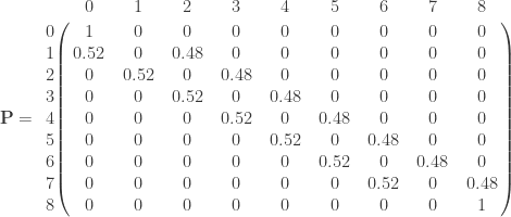
Example 4 (Gambler’s Ruin)
Consider a small scaled gambler’s ruin problem. Say, $N=8$ and $p=0.48$ . That is, the gambler makes a series of one-unit bets against the house such that the probability of winning a bet is 0.48 and such that the gambler stops whenever his total capital is 0 units (the gambler is in ruin) or 8 units.

Let $X_n$ be the gambler’s capital (the number of units) after the $n$ th bet. The following is the transition probability matrix describing this Markov chain.

$\mathbf{P} = \bordermatrix{ & 0 & 1 & 2 & 3 & 4 & 5 & 6 & 7 & 8 \cr 0 & 1 & 0 & 0 & 0 & 0 & 0 & 0 & 0 & 0 \cr 1 & 0.52 & 0 & 0.48 & 0 & 0 & 0 & 0 & 0 & 0 \cr 2 & 0 & 0.52 & 0 & 0.48 & 0 & 0 & 0 & 0 & 0 \cr 3 & 0 & 0 & 0.52 & 0 & 0.48 & 0 & 0 & 0 & 0 \cr 4 & 0 & 0 & 0 & 0.52 & 0 & 0.48 & 0 & 0 & 0 \cr 5 & 0 & 0 & 0 & 0 & 0.52 & 0 & 0.48 & 0 & 0 \cr 6 & 0 & 0 & 0 & 0 & 0 & 0.52 & 0 & 0.48 & 0 \cr 7 & 0 & 0 & 0 & 0 & 0 & 0 & 0.52 & 0 & 0.48 \cr 8 & 0 & 0 & 0 & 0 & 0 & 0 & 0 & 0 & 1 \cr } \qquad$

There are two absorbing states in this chain, state 0 and state 8 (ruin or winning all units). The transient states are 1, 2, 3, 4, 5, 6 and 7. As discussed in this post, $Q$ is the matrix consisting of all transition probabilities $P_{ij}$ from the transient states into the transient states. Then derive the matrix $I-Q$ and compute its inverse.

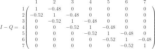
$I-Q = \bordermatrix{ & 1 & 2 & 3 & 4 & 5 & 6 & 7 \cr 1 & 1 & -0.48 & 0 & 0 & 0 & 0 & 0 \cr 2 & -0.52 & 1 & -0.48 & 0 & 0 & 0 & 0 \cr 3 & 0 & -0.52 & 1 & -0.48 & 0 & 0 & 0 \cr 4 & 0 & 0 & -0.52 & 1 & -0.48 & 0 & 0 \cr 5 & 0 & 0 & 0 & -0.52 & 1 & -0.48 & 0 \cr 6 & 0 & 0 & 0 & 0 & -0.52 & 1 & -0.48 \cr 7 & 0 & 0 & 0 & 0 & 0 & -0.52 & 1 \cr } \qquad$

$W=(I-Q)^{-1} = \bordermatrix{ & 1 & 2 & 3 & 4 & 5 & 6 & 7 \cr 1 & 1.7444 & 1.4316 & 1.1429 & 0.8763 & 0.6303 & 0.4032 & 0.1935 \cr 2 & 1.5509 & 2.9825 & 2.3810 & 1.8257 & 1.3131 & 0.8399 & 0.4032 \cr 3 & 1.3413 & 2.5794 & 3.7223 & 2.8541 & 2.0528 & 1.3131 & 0.6303 \cr 4 & 1.1142 & 2.1426 & 3.0920 & 3.9683 & 2.8541 & 1.8257 & 0.8763 \cr 5 & 0.8681 & 1.6695 & 2.4092 & 3.0920 & 3.7223 & 2.3810 & 1.1429 \cr 6 & 0.6016 & 1.1569 & 1.6695 & 2.1426 & 2.5794 & 2.9825 & 1.4316 \cr 7 & 0.3128 & 0.6016 & 0.8681 & 0.1142 & 1.3413 & 1.5509 & 1.7444 \cr } \qquad$

The fundamental matrix $(I-Q)^{-1}$ gives a wealth of information about the prospect for the gambler in question. Suppose the gambler initially has 3 units in capital. The sum of the third row is 14.49, roughly 14.5. So on average the gambler makes 14.5 bets before reaching one of the two absorbing states (in ruin or owning all 8 units). With one bet = one period of time, the gambler spends on average 3.72 periods of time in state 3. Note that most of the time the gambler is in the lower capital states. The gambler that has initially 3 units only spends on average 0.6303 amount of time in state 7, an indication that the gambler does not have a great chance of winning all 8 units.

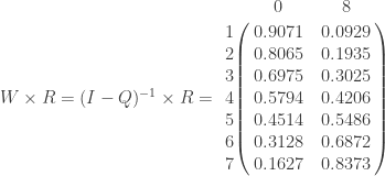
The matrix $W \times R$ gives the probabilities of absorption.

$R = \bordermatrix{ & 0 & 8 \cr 1 & 0.52 & 0 \cr 2 & 0 & 0 \cr 3 & 0 & 0 \cr 4 & 0 & 0 \cr 5 & 0 & 0 \cr 6 & 0 & 0 \cr 7 & 0 & 0.48 \cr } \qquad$

$W \times R = (I-Q)^{-1} \times R= \bordermatrix{ & 0 & 8 \cr 1 & 0.9071 & 0.0929 \cr 2 & 0.8065 & 0.1935 \cr 3 & 0.6975 & 0.3025 \cr 4 & 0.5794 & 0.4206 \cr 5 & 0.4514 & 0.5486 \cr 6 & 0.3128 & 0.6872 \cr 7 & 0.1627 & 0.8373 \cr } \qquad$

The first column of $W \times R$ gives the probabilities of ruin for the gambler. The smaller the initial capital, the greater the probability of ruin. With 3 units initially, the gambler has an almost 70% chance of ruin.

More about Fundamental Matrix

The fundamental matrix of an absorbing Markov chain is central to the technique described here. We now attempt to give an indication why the technique works.

Let $\mathbf{P}$ be the transition probability transition matrix for an absorbing Markov chain. Suppose that $\mathbf{P}$ is stated as follows

$\mathbf{P}=\left[\begin{array}{rr} Q & R \\ \mathbf{0} & I \\ \end{array}\right]$

such that $Q$ is the submatrix of $\mathbf{P}$ that consists of the one-step transition probabilities between transient states and $R$ is the submatrix of $\mathbf{P}$ that consists of the one-step transition probabilities from transient states into absorbing states. The fundamental matrix is $W=(I-Q)^{-1}$ , which is the inverse of the matrix $I-Q$ where $I$ is the identity matrix of the same size as $Q$ .

We sketch an answer to two questions. Why each entry $W_{ij}$ in the fundamental matrix $W$ is the mean time the process spent in state $j$ given that the process starts in state $i$ ? Why the matrix $W \times R$ gives the probabilities of absorption?

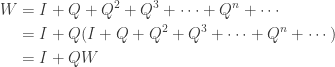
Note that the entries in $Q^n$ , the $n$ th power of the matrix $Q$ , approach zero as $n$ becomes large. This is because $Q$ contains the one-step transition probabilities of the transient states (once in a transient state, the process has to leave the transient states at some point). We have the following equality.

$W=I+Q+Q^2+Q^3+\cdots+Q^n+\cdots \ \ \ \ \ \ \ \ \ \ \ \ \ \ \ \ \ \ \ \ \ \ \ \ \ \ \ \ \ \ (3)$

To see the equality (3), fix transient states $i$ and $j$ with $i \ne j$ . We show the following:

$W_{ii}=1+P_{ii}+P_{ii}^2+P_{ii}^3+\cdots+P_{ii}^n+\cdots \ \ \ \ \ \ \ \ \ \ \ \ \ \ \ \ \ \ \ \ \ \ \ \ \ \ \ \ \ (4)$

$W_{ij}=P_{ij}+P_{ij}^2+P_{ij}^3+\cdots+P_{ij}^n+\cdots \ \ \ \ \ \ \ \ \ \ \ \ \ \ \ \ \ \ \ \ \ \ \ \ \ \ \ \ \ \ \ \ \ (5)$

Suppose the process starts at state $i$ . Define the indicator variables $Y_n$ and $Z_n$ for $n \ge 1$ . At time $n$ , if the process is in state $i$ , let $Y_n=1$ . Otherwise $Y_n=0$ . Likewise, at time $n$ , if the process is in state $j$ , let $Z_n=1$ . Otherwise $Z_n=0$ . By definition,

$\displaystyle 1+Y_1+Y_2+Y_3+\cdots+Y_n+\cdots$

$\displaystyle Z_1+Z_2+Z_3+\cdots+Z_n+\cdots$

are the times spent in state $i$ and in state $j$ , respectively. The 1 in the first random time accounts for the fact that the process is already in state $i$ initially. Because we are dealing with transient states, only a finite number of $Y_n$ and $Z_n$ can be 1’s. So these two random time variables are well defined. Each $Y_n$ is a Bernoulli random variable with $P[Y_n=1]=P_{ii}^n$ . Likewise each $Z_n$ is a Bernoulli random variable with $P[Z_n=1]=P_{ij}^n$ . The following gives (4) and (5).

$\displaystyle \begin{aligned} W_{ii}&=1+E[Y_1]+E[Y_2]+\cdots+E[Y_n]+\cdots \\&=1+P_{ii}+P_{ii}^2+\cdots+P_{ii}^n+\cdots \end{aligned}$

$\displaystyle \begin{aligned} W_{ij}&=E[Z_1]+E[Z_2]+\cdots+E[Z_n]+\cdots \\&=P_{ij}+P_{ij}^2+\cdots+P_{ij}^n+\cdots \end{aligned}$

Expressing equalities (4) and (5) in matrix form gives the equality (3). The following derivation shows that $W=(I-Q)^{-1}$ .

$\displaystyle \begin{aligned} W&=I+Q+Q^2+Q^3+\cdots+Q^n+\cdots \\&=I+Q (I+Q+Q^2+Q^3+\cdots+Q^n+\cdots) \\& = I+ Q W\end{aligned}$

$W-Q W=I$

$W (I-Q)=I$

Thus the mean times spent in the transient states are obtained by taking the inverse of the matrix $I-Q$ . Based on the derivation, the sum $I+Q+Q^2+Q^3+\cdots+Q^n$ for a sufficiently large $n$ would give a good approximation of the waiting time matrix $W$ . Of course, computationally speaking, it is much easier to compute the inverse matrix of $I-Q$ .

For the second question, it is instructive to examine the power of $\mathbf{P}$ . By induction on the power $n$ , $\mathbf{P}^n$ can be expressed as follows:

$\mathbf{P}^n=\left[\begin{array}{rr} Q^n & M_n \\ \mathbf{0} & I \\ \end{array}\right]=\left[\begin{array}{rr} Q^n & (I+Q+Q^2+Q^3+\cdots+Q^{n-1}) R \\ \mathbf{0} & I \\ \end{array}\right]$

The entries in the matrix $M_n$ are the $n$ -step transition probabilities from a transient state to an absorbing state. For example, if the starting state is the transient state $i$ and $k$ is an absorbing state, then $P_{ik}^n$ is an entry of $M_n=(I+Q+Q^2+Q^3+\cdots+Q^{n-1}) R$ . Starting at a transient state, the process will be absorbed at some point in time. So the matrix $M_n$ gives good approximation for probabilities of absorption when $n$ is large. Note that $M_n=(I+Q+Q^2+Q^3+\cdots+Q^{n-1}) R$ approaches $W \times R$ as $n$ goes to infinity.

The type of Markov chains discussed here are called absorbing Markov chains, the subject of next post.

Practice Problems

Practice problems to reinforce the concepts discussed here are available in a companion blog. There are two problem sets. The first one is here and the second one is here.

Dan Ma Markov chains

Daniel Ma Markov chains

Topics in Probability

concepts in applied probability

Monthly Archives: December 2017

First step analysis and fundamental matrix